Plotting eight centuries of river discharge in Asia
/ Hung Nguyen
Introduction
Figure 1 below is a complex plot, with multiple panels and annotations, that was created fully in R. Initially, I made the main figure in R and annotated it in Adobe Acrobat. But soon I got tired of re-annotating the figure every time I revised it. So I put in some effort to make the whole plot completely reproducible. In this post, I will detail the steps to create this figure. Rather than showing just the good working code, I will try to describe some of my thinking process to show how the plot developed through trial and error.
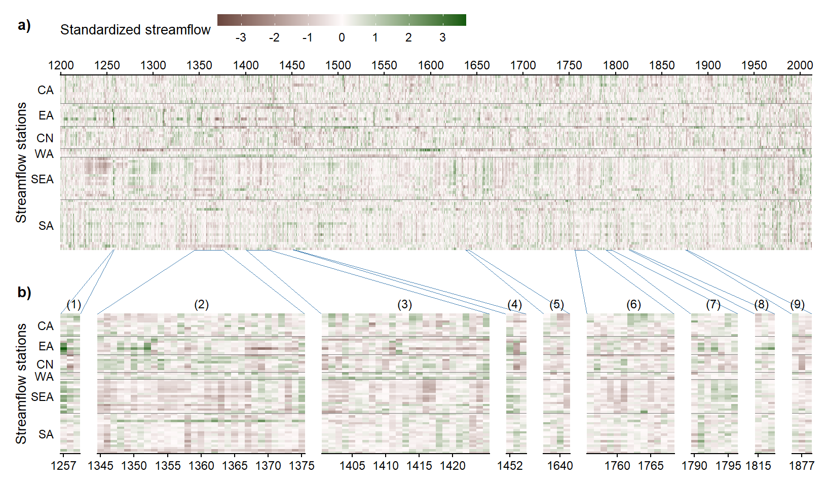
Figure 1. Eight centuries of river discharge history in Asia. Panel a shows the standardized streamflow index (SSI, the z-score of the annual discharge) at 62 rivers in Asia. Negative SSI values correspond to low flow (dry conditions) and positive SSI values denote high flow (wet conditions). The rivers are divided into six regions: CA (Central Asia), EA (East Asia), CN (eastern China), WA (West Asia), SEA (Southeast Asia), and SA (South Asia). Panel b shows the SSI in nine historical events: (1) the Samalas eruption, (2) and (3) the Angkor Droughts I and II, (4) the Kuwae eruption, (5) the Ming Dynasty Drought, (6) the Strange Parallel Drought, (7) the East India Drought, (8) the Tambora eruption, and (9) the Victorian Great Drought. Refer to (Nguyen et al. 2020) for more details.
The stations’ locations are provided in Figure 2.
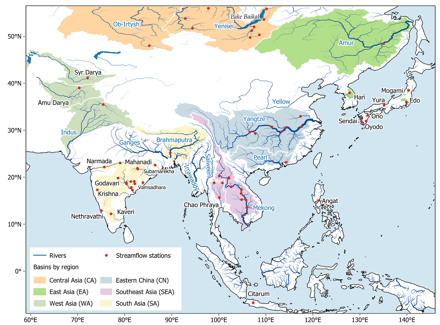
Figure 2. Map of the discharge stations and their river basins.
Data
The data are provided in the GitHub repo of this blog. Let’s read the file and have an overview of the data.
library(data.table)
ssi <- fread('asia-standardiized-streamflow-index.csv', key = 'ID')
ssi
## ID year ssi
## 1: BD_0000001 1200 -0.2381706
## 2: BD_0000001 1201 -1.0028535
## 3: BD_0000001 1202 -0.2155856
## 4: BD_0000001 1203 -0.1527892
## 5: BD_0000001 1204 -0.2537824
## ---
## 50402: TJ_0000003 2008 0.2308875
## 50403: TJ_0000003 2009 -0.1633646
## 50404: TJ_0000003 2010 1.3372388
## 50405: TJ_0000003 2011 1.1759821
## 50406: TJ_0000003 2012 -0.7078168The data already come in the tidy format, so that’s great.
range(ssi$ssi)## [1] -2.940408 3.691093I’ve also provided the metadata for the stations. Let’s take a look.
meta <- fread('station-meta.csv', key = 'ID')
head(meta, 10)
## ID region basin river name long lat
## 1: BD_0000001 SA Brahmaputra Brahmaputra Bahadurabad 89.69582 25.179169
## 2: CN_0000180 CN Yangtze Yangtze Datong 117.62082 30.770836
## 3: CN_0000181 CN Yangtze Huai He Bengbu 117.36249 32.954169
## 4: CN_0000189 CN Pearl Dong Jiang Boluo 114.30415 23.162503
## 5: CN_0000190 CN Yangtze Yangtze Cuntan 106.59582 29.612502
## 6: CN_0000191 CN Yangtze Yangtze Hankou 114.29582 30.579169
## 7: CN_0000192 CN Yangtze Yangtze Luoshan 113.34582 29.687502
## 8: CN_0000194 CN Yangtze Yangtze Wulong 107.76249 29.320836
## 9: CN_0000195 CN Yangtze Yangtze Yichang 111.27916 30.695836
## 10: ID_0000024 SEA Citarum Citarum Citarum 107.29420 -6.730795Plotting panel a
First, let’s plot the basic heat map.
library(ggplot2)
ggplot(ssi) +
  geom_raster(aes(year, ID, fill = ssi)) +
  scale_x_continuous(
    name = NULL,
    breaks = seq(1200, 2000, 50),
    expand = c(0, 0),
    position = 'top') +
  scale_y_discrete(name = 'Streamflow station', expand = c(0, 0)) +
  scale_fill_gradient2(
    name = 'Standardized streamflow index',
    low = '#6b473e', mid = 'snow1', high = '#125a0d',
    breaks = -3:3,
    limits = c(-3.7, 3.7)) +
  theme(
    legend.key.width = unit(1, 'cm'),
    legend.key.height = unit(0.3, 'cm'),
    legend.justification = 'left',
    legend.position = 'top',
    axis.line.x = element_line())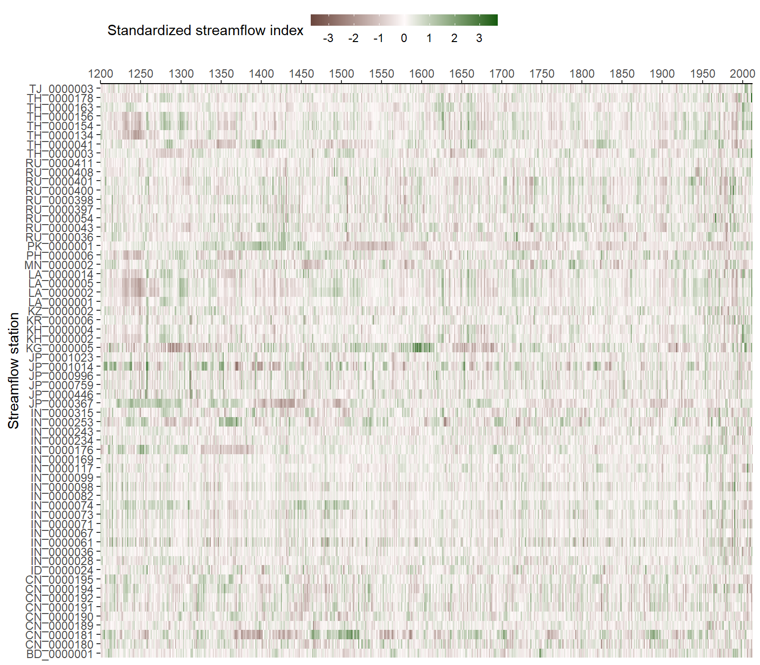
The heat map looks good. However, the stations are arranged by alphabetical order, which is not what we want. They should be arranged by region, and from South to North in each region (South to North rather than North to South because when plotting, the y-axis goes up). So the next step is to arrange the stations using their metadata.
# First, we arrange the regions from South to North
meta[, region := factor(region, c('SA', 'SEA', 'WA', 'CN', 'EA', 'CA'))]
# Now we sort by region and lattitude
meta <- meta[order(region, lat)]
# Now we create a column code to encode the plotting order
meta[, plotOrder := 1:.N]
# Let's insepct the updated meta, showing only the columns of interest
print(meta[, .(ID, region, lat, plotOrder)], nrows = 50)
## ID region lat plotOrder
## 1: IN_0000176 SA 12.18920 1
## 2: IN_0000315 SA 12.88440 2
## 3: IN_0000098 SA 17.25190 3
## 4: IN_0000117 SA 17.29584 4
## 5: IN_0000099 SA 17.79890 5
## ---
## 58: RU_0000043 CA 52.02083 58
## 59: RU_0000398 CA 53.59583 59
## 60: RU_0000411 CA 53.79583 60
## 61: RU_0000397 CA 55.84583 61
## 62: RU_0000408 CA 55.96250 62Let’s merge the data now so that we can rearrange the stations in the plot.
# Merge by ID
ssi2 <- merge(ssi, meta[, .(ID, region, plotOrder)], by = 'ID')
# Plot
ggplot(ssi2) +
  geom_raster(aes(year, plotOrder, fill = ssi)) +
  scale_x_continuous(
    name = NULL,
    breaks = seq(1200, 2000, 50),
    expand = c(0, 0),
    position = 'top') +
  # y-axis is now continous (plot order) instead of discrete (ID)
  scale_y_continuous(
    name = 'Streamflow station',
    expand = c(0, 0)) +
  scale_fill_gradient2(
    name = 'Standardized streamflow index',
    low = '#6b473e', mid = 'snow1', high = '#125a0d',
    breaks = -3:3,
    limits = c(-3.7, 3.7)) +
  theme(
    legend.key.width = unit(1, 'cm'),
    legend.key.height = unit(0.3, 'cm'),
    legend.justification = 'left',
    legend.position = 'top',
    axis.line.x = element_line())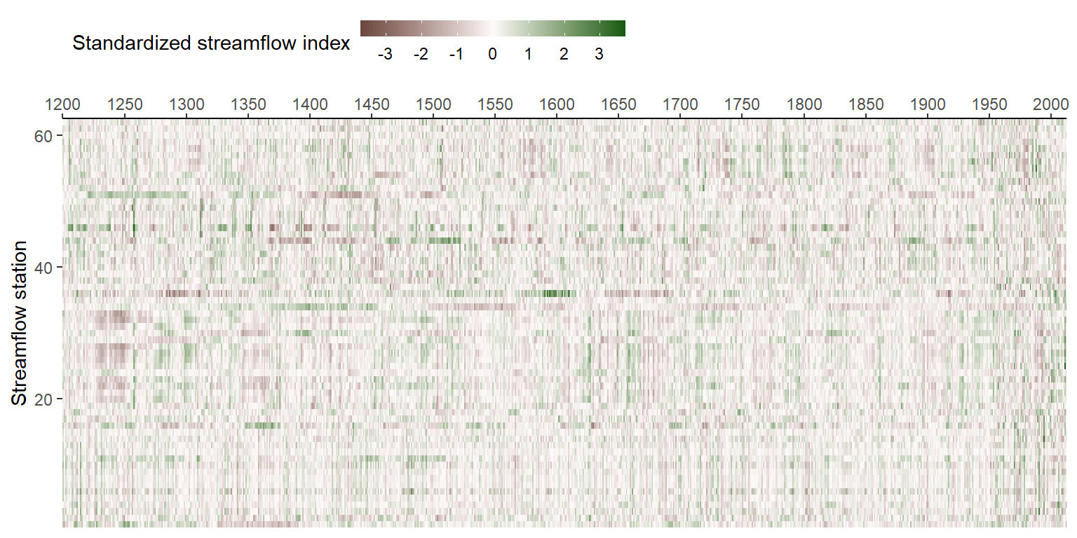
Now the stations are in order. The next step is to plot the region delination lines, hide away the order number, and annotate with the region names instead. To do so, we need to determine the vertical locations of the region lines and texts.
# Determine the number of stations in each region
regions <- meta[, .(count = .N), by = region]
# Starting point for lines. Each cell has size 1x1,
# therefore we add 0.5 so that the lines are at the top of the cells.
regions[1, top := count + 0.5]
for (i in 2:nrow(regions)) regions$top[i] <- regions$top[i-1] + regions$count[i]
# Midpoints for annotation
regions[, mid := top - count / 2]
We can now plot with annotations.
ggplot(ssi2) +
  geom_raster(aes(year, plotOrder, fill = ssi)) +
  # Plot the region delination lines
  geom_hline(aes(yintercept = top), regions, colour = 'grey50') +
  annotate(
    geom = 'text',
    x = 1150,  # Extend the x-axis back to the left
    y = regions$mid,
    label = regions$region,
    hjust = 0) +
  scale_x_continuous(
    name = NULL,
    breaks = seq(1200, 2000, 50),
    expand = c(0, 0),
    position = 'top') +
  scale_y_continuous(
    name = 'Streamflow station',
    expand = c(0, 0)) +
  scale_fill_gradient2(
    name = 'Standardized streamflow index',
    low = '#6b473e', mid = 'snow1', high = '#125a0d',
    breaks = -3:3,
    limits = c(-3.7, 3.7)) +
  theme(
    # Because we extended the axis back,
    # there is now a grey background (ggplot2 default)
    # We need to remove it
    panel.background = element_blank(),
    legend.key.width = unit(1, 'cm'),
    legend.key.height = unit(0.3, 'cm'),
    legend.justification = 'left',
    legend.position = 'top',
    axis.line.x = element_line(),
    # Remove the y-axis text and ticks
    axis.text.y = element_blank(),
axis.ticks.y = element_blank()) 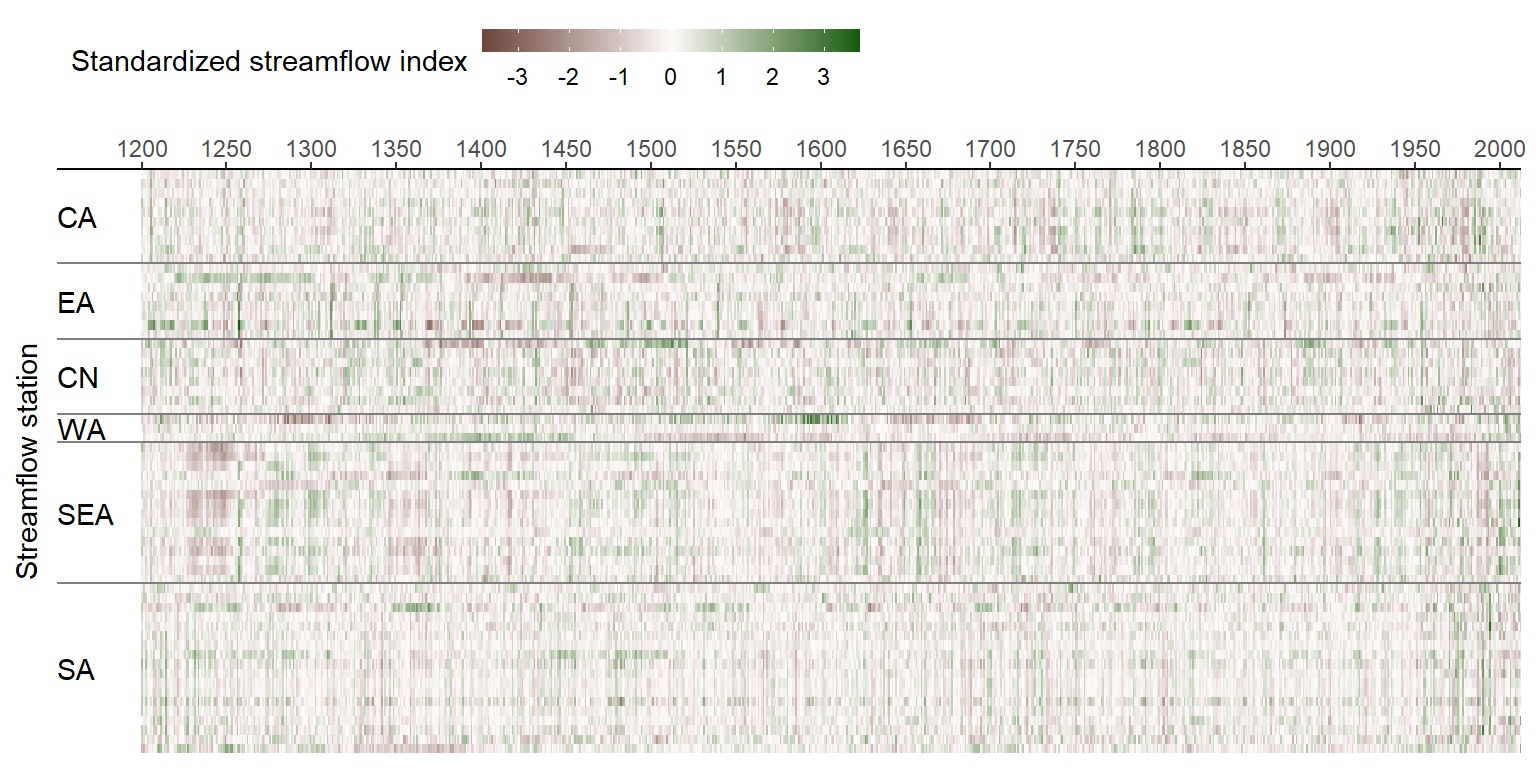
Now the region lines and the texts are where they need to be, but the lines extend too far to the left. We extended the x-axis back to the year 1150 so that we could plot the region texts, and we used geom_hline(), which draws lines throughout the plot. We could fix this by changing from geom_hline() to geom_linerange() and providing additional xmax and xmin arguments. I tried this and realized that this didn’t work because the x-axis still extended back and that looked ugly. Then I came up with a new trick: I’ll make use of the axis breaks for the region texts. This way, I don’t have to extend the x-axis back, and I don’t have to add a new layer.
ggplot(ssi2) +
  geom_raster(aes(year, plotOrder, fill = ssi)) +
  # Keep geom_hline()
  geom_hline(aes(yintercept = top), regions, colour = 'grey50') +
  scale_x_continuous(
    name = NULL,
    breaks = seq(1200, 2000, 50),
    expand = c(0, 0),
    position = 'top') +
  scale_y_continuous(
    name = 'Streamflow station',
    # Add breaks and break labels
    breaks = regions$mid,
    labels = regions$region,
    expand = c(0, 0)) +
  scale_fill_gradient2(
    name = 'Standardized streamflow index',
    low = '#6b473e', mid = 'snow1', high = '#125a0d',
    breaks = -3:3,
    limits = c(-3.7, 3.7)) +
  theme(
    panel.background = element_blank(),
    legend.key.width = unit(1, 'cm'),
    legend.key.height = unit(0.3, 'cm'),
    legend.justification = 'left',
    legend.position = 'top',
    axis.line.x = element_line(),
    # the line axis.text.y = element_blank() is removed
axis.ticks.y = element_blank()) 
Hooray!
Plotting panel b
Panel b consists of subsets of panel a for different periods. Thus we can transform the code of panel a into a function that takes the starting and ending years and just plots the heatmap for that period. Additionally, we need to take care of the axes: panel a’s x-axis is on top while those of panel b is at the bottom, and the x-axis has custom breaks. Only the first subpanel of b has the region texts. Only panel a has the legend. These options can be handled easily by function aruguments.
Plotting routine
flow_history <- function(ssi.data,
                         region.data,
                         start.year,
                         end.year,
                         legend.position = c('top', 'none'),
                         x.breaks,
                         x.axis.position = c('bottom', 'top'),
                         region.text = FALSE) {
  # Filter the data by year
  ggplot(ssi.data[year %between% c(start.year, end.year)]) +
    geom_raster(aes(year, plotOrder, fill = ssi)) +
    geom_hline(aes(yintercept = top), region.data, colour = 'grey50') +
    scale_x_continuous(
      name = NULL,
      # custom x breaks
      breaks = x.breaks,
      expand = c(0, 0),
      # custom axis position (bottom or top)
      position = x.axis.position) +
    scale_y_continuous(
      name = 'Streamflow station',
      breaks = region.data$mid,
      labels = region.data$region,
      expand = c(0, 0)) +
    scale_fill_gradient2(
      name = 'Standardized streamflow index',
      low = '#6b473e', mid = 'snow1', high = '#125a0d',
      na.value = 'white',
      breaks = -3:3,
      limits = c(-3.7, 3.7)) +
    theme(
      panel.background = element_blank(),
      legend.key.width = unit(1, 'cm'),
      legend.key.height = unit(0.3, 'cm'),
      legend.justification = 'left',
      legend.position = legend.position,
      axis.line.x = element_line(),
      # Whether to show region texts
      axis.text.y = if (!region.text) element_blank(),
      # Whether to show y-axis title (hidden if region texts are not shown)
      axis.title.y = if (!region.text) element_blank() else element_text(angle = 90),
      axis.ticks.y = element_blank())
}
Now let’s test this function.
# Panel a: full plot
pa <- flow_history(
  ssi.data = ssi2, region.data = regions,
  # Full time horizon
  start.year = 1200, end.year = 2012,
  legend.position = 'top',
  x.breaks = seq(1200, 2000, 50),
  x.axis.position = 'top',
  region.text = TRUE)
pa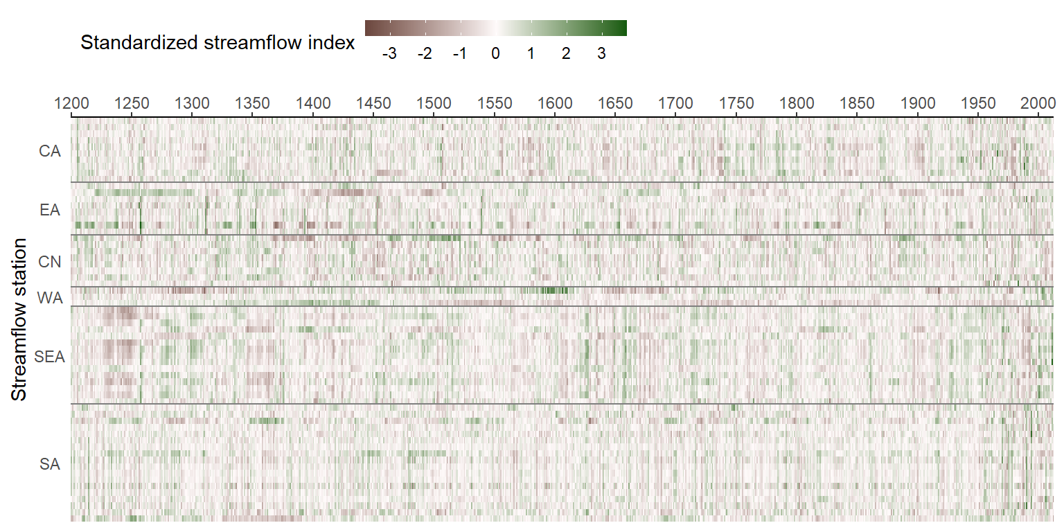
# Panel b1: Samalas eruption
pb1 <- flow_history(
  ssi.data = ssi2, region.data = regions,
  # 3 years surrounding the event
  start.year = 1257, end.year = 1259,
  legend.position = 'none',
  x.breaks = 1258,
  x.axis.position = 'bottom',
  region.text = TRUE)
pb1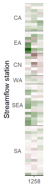
# Panel b2: Angkor Drought I
pb2 <- flow_history(
  ssi.data = ssi2, region.data = regions,
  start.year = 1345, end.year = 1375,
  legend.position = 'none',
  x.breaks = seq(1345, 1375, 5),
  x.axis.position = 'bottom',
  region.text = FALSE)
pb2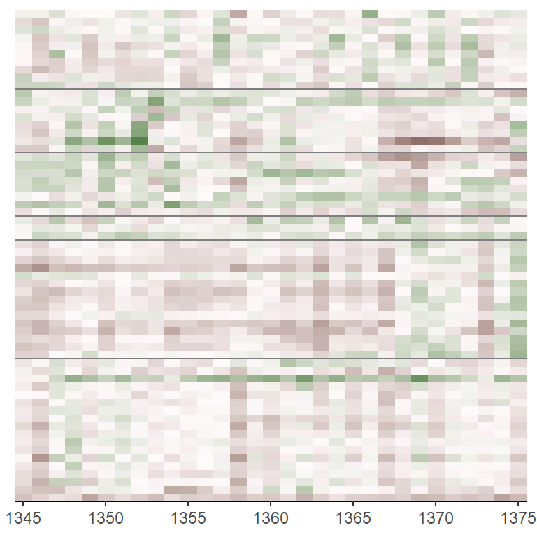
Now that the individual panels can be plotted, let’s assemble them.
Assembling plots
There are many packages to assemble plots, perhaps the most common of which are cowplot by Claus O. Wilke and patchwork by Thomas Lin Pedersen. The two packages work a bit differently. I think the aspect most relevant to our task here is the way the packages scale the width and height of the plots. cowplot includes the axes when calculating widths and heights while patchwork doesn’t. To visualize this difference, let’s put panels b1 and b2 together using these two packages. There are 3 years in panel b1 and 21 years in panel b2, so we’ll scale them with the ratio 3/31.
# Assemble with cowplot
library(cowplot)
plot_grid(pb1, pb2, rel_widths = c(3, 31))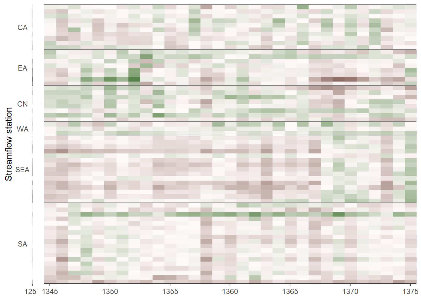
# Assemble with patchwork
library(patchwork)
pb1 + pb2 +
  plot_layout(widths = c(3, 31))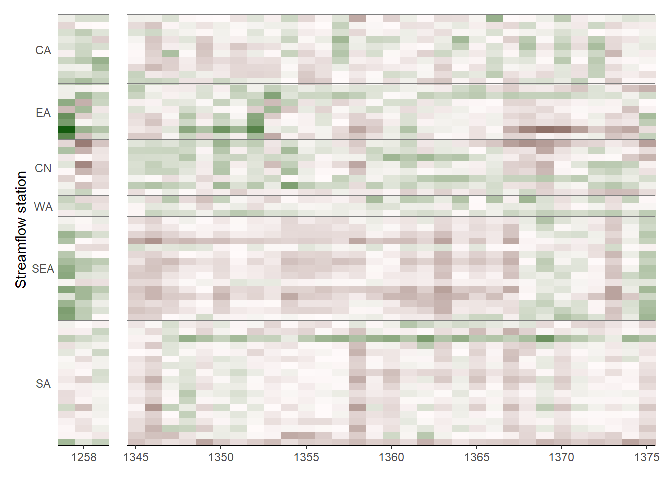
Notice what happens to b1. Because cowplot counts the y-axis when calculating plot width, and b1 has a wide y-axis and b2 does not, b1 gets squished. patchwork only considers the plot body for widths, so this problem does not happen.
Let’s now make the rest of panel b and then assemble.
# Panels b3 to b9
pb3 <- flow_history(ssi2, regions, 1401, 1425, x.breaks = seq(1405, 1420, 5),
                    legend.position = 'none', x.axis.position = 'bottom')
pb4 <- flow_history(ssi2, regions, 1452, 1454, x.breaks = 1452,
                    legend.position = 'none', x.axis.position = 'bottom')
pb5 <- flow_history(ssi2, regions, 1638, 1641, x.breaks = 1640,
                    legend.position = 'none', x.axis.position = 'bottom')
pb6 <- flow_history(ssi2, regions, 1756, 1768, x.breaks = c(1760, 1765),
                    legend.position = 'none', x.axis.position = 'bottom')
pb7 <- flow_history(ssi2, regions, 1790, 1796, x.breaks = c(1790, 1795),
                    legend.position = 'none', x.axis.position = 'bottom')
pb8 <- flow_history(ssi2, regions, 1815, 1817, x.breaks = 1815,
                    legend.position = 'none', x.axis.position = 'bottom')
pb9 <- flow_history(ssi2, regions, 1876, 1878, x.breaks = 1877,
                    legend.position = 'none', x.axis.position = 'bottom')
# Panel b together
pb <- pb1 + pb2 + pb3 + pb4 + pb5 + pb6 + pb7 + pb8 + pb9 +
  # Set relative widths based on the number of years in each period
  plot_layout(widths = c(3, 31, 25, 3, 4, 13, 7, 3, 3), nrow = 1)
# Merging panels a and b
pab <- pa + plot_spacer() + pb +
  plot_layout(ncol = 1, heights = c(1, 0.2, 0.8))
pab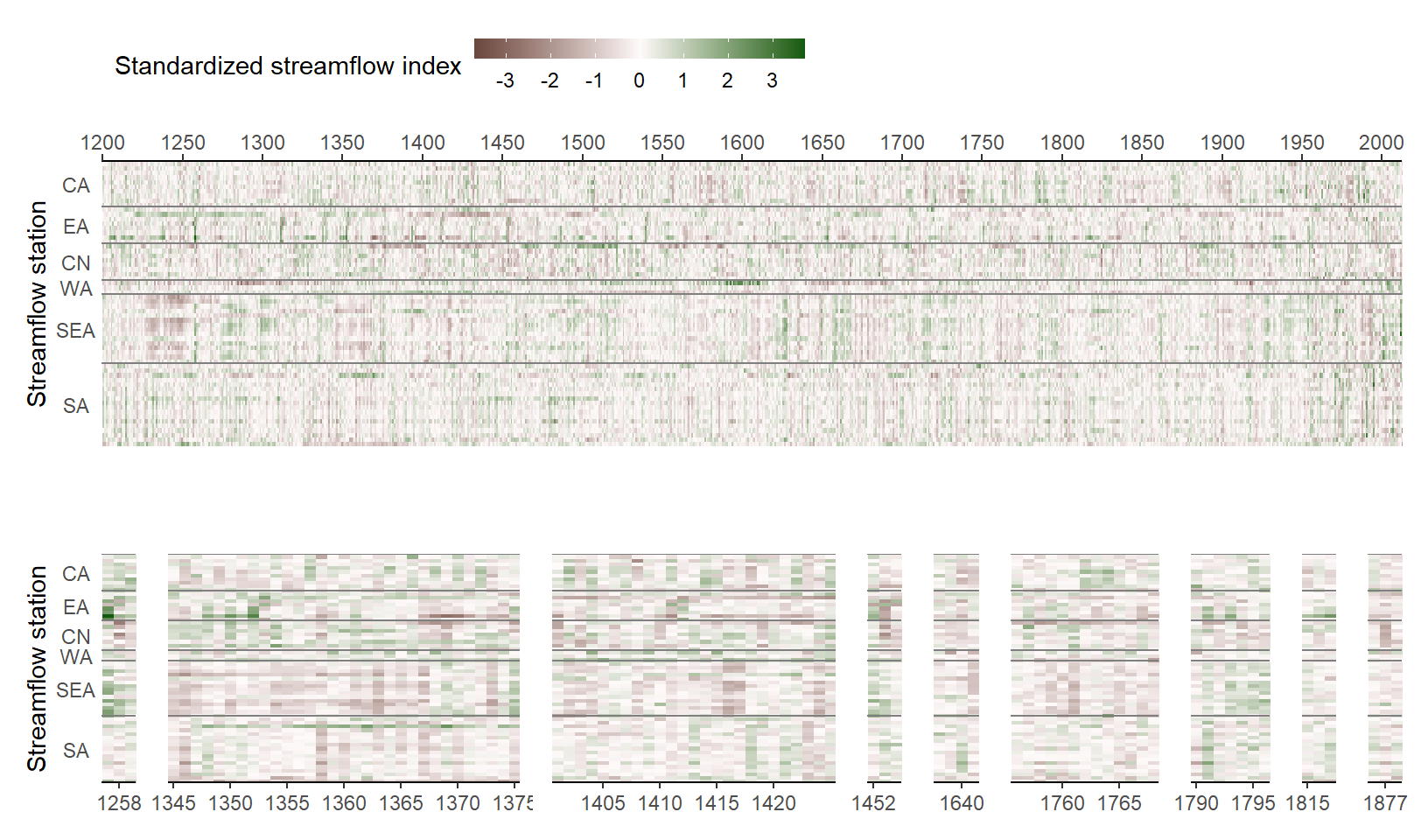
We have the plot! Now all we need to do is add the annotations.
Annotating
The horizontal lines at the bottom of panel a is easy to do with geom_segment().
# Starting and ending years of events
segments <- data.table(
  x    = c(1257, 1345, 1401, 1452, 1638, 1756, 1790, 1815, 1876),
  xend = c(1258, 1375, 1425, 1453, 1641, 1768, 1796, 1816, 1878))
# Add the segments to panel a
pa <- pa +
  geom_segment(aes(x = x, xend = xend, y = 0.125, yend = 0.125), size = 0.4,
                   data = segments, colour = 'steelblue')
# Update the assembly
pab <- pa + plot_spacer() + pb +
  plot_layout(ncol = 1, heights = c(1, 0.2, 0.8))
pab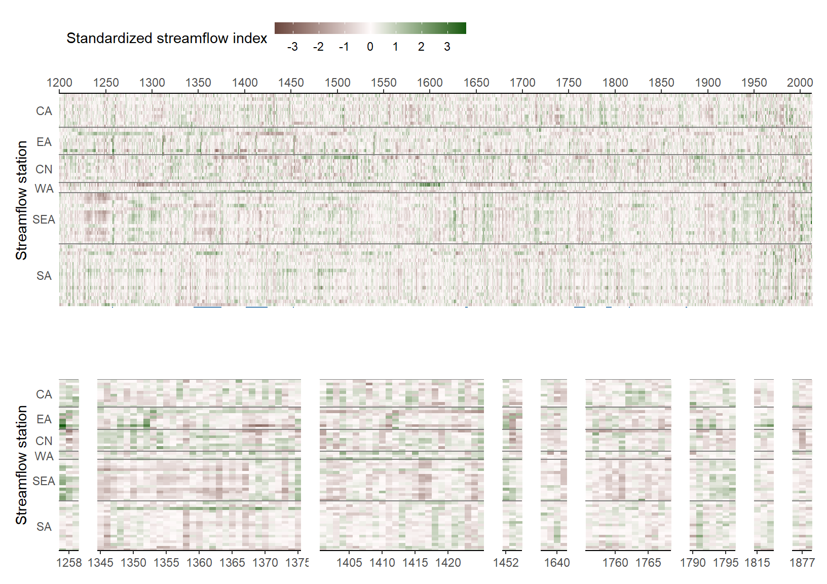
Drawing the lines connecting the panels is more challenging. The annotations link different panels, and it’s rather difficult to determine their relative positions, because each panel has its own coordinate system. Instead, I transformed them into one grid object with one coordinate system, and drew the annotations on this canvas. This was possible thanks to cowplot.
# Transform the patchwork into a grid object
fhGrob <- patchwork::patchworkGrob(pab)
# Draw tthe grid object as a cowplot object
fhWrap <- cowplot::ggdraw(fhGrob)
Now I just need to determine the positions of the lines nad texts. This was relatively easy because I knew the starting and ending years of each event, so I could determine the proportions of the lines. Still, it took some trying and adjusting. Finally, these numbers below work for a 8.5 in x 6 in canvas.
yLine <- c(0.3500, 0.4730)
yText <- 0.365

fhAnnotated <- fhWrap +
  # Each event has two marking lines for the start and the end
  draw_line(c(0.0730, 0.1370), yLine, colour = 'steelblue', size = 0.4) + #1
  draw_line(c(0.0970, 0.1380), yLine, colour = 'steelblue', size = 0.4) + #1
  draw_line(c(0.1180, 0.2360), yLine, colour = 'steelblue', size = 0.4) + #2
  draw_line(c(0.3685, 0.2690), yLine, colour = 'steelblue', size = 0.4) + #2
  draw_line(c(0.3890, 0.2975), yLine, colour = 'steelblue', size = 0.4) + #3
  draw_line(c(0.5925, 0.3245), yLine, colour = 'steelblue', size = 0.4) + #3
  draw_line(c(0.6120, 0.3545), yLine, colour = 'steelblue', size = 0.4) + #4
  draw_line(c(0.6361, 0.3560), yLine, colour = 'steelblue', size = 0.4) + #4
  draw_line(c(0.6575, 0.5625), yLine, colour = 'steelblue', size = 0.4) + #5
  draw_line(c(0.6892, 0.5664), yLine, colour = 'steelblue', size = 0.4) + #5
  draw_line(c(0.7100, 0.6950), yLine, colour = 'steelblue', size = 0.4) + #6
  draw_line(c(0.8150, 0.7085), yLine, colour = 'steelblue', size = 0.4) + #6
  draw_line(c(0.8355, 0.7325), yLine, colour = 'steelblue', size = 0.4) + #7
  draw_line(c(0.8925, 0.7392), yLine, colour = 'steelblue', size = 0.4) + #7
  draw_line(c(0.9128, 0.7610), yLine, colour = 'steelblue', size = 0.4) + #8
  draw_line(c(0.9371, 0.7625), yLine, colour = 'steelblue', size = 0.4) + #8
  draw_line(c(0.9575, 0.8290), yLine, colour = 'steelblue', size = 0.4) + #9
  draw_line(c(0.9820, 0.8308), yLine, colour = 'steelblue', size = 0.4) + #9
  # Event numbers
  draw_text(paste0('(', 1:9, ')'),
            c(0.090, 0.244, 0.490, 0.623, 0.674, 0.767, 0.863, 0.921, 0.965),
            yText, size = 9) +
  # Panel tag
  draw_text(c('a)', 'b)'), 0.03, c(0.95, 0.4), size = 11, fontface = 'bold')
fhAnnotated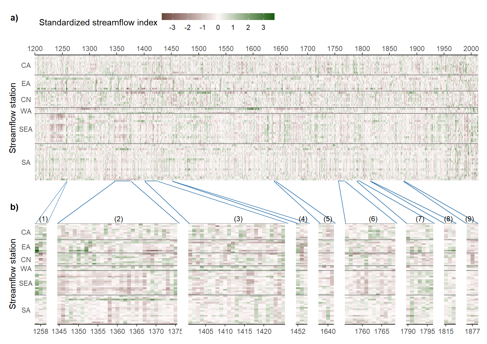
Summary
In creating this complex plot, we’ve gone through several stages. Let’s recap.
- First, we wrote a routine to create the overall plot (panel a)
- Then, we converted that routine into a function with arguments for time period and layout, so that we can create multiple plots for sub-periods (panel b)
- We assembled the panels with
patchwork. This yielded apatchworkobject. - We converted the
patchworkobject into a genericgrobthat could be read intocowplot. - The
grobacted as a canvas onwhich we drew the annotations.
This post has demonstrated how a complex plot can be built up from the pieces. I hope it’ll be useful for your next visualization.