Hourly power generation at US dams

May 23, 2020 /

Some time ago I sent out a message to energy Twitter to see whether hourly-resolution data for US dams are publicly available anywhere.

I had no luck, but since then I’ve come across a couple of useful resources. It’s possible to get hourly generation (MW) records for a handful of dams in the Columbia River Basin though the US Army Corps of Engineers. And you can powered releases (cfs) handful of dams in the Upper Colorado via the US Bureau of Reclamation. Powered release is simply the flow through the turbines. This isn’t quite the same as generation, but one can reasonably estimate generation from release with knowledge of hydraulic head and turbine efficiency.

Here’s a quick tutorial for how to download and wrangle both datasets.

1. USACE power generation records (Pacific Northwest)

If you search the USACE data portal for “Grand Coulee” you’ll be presented with an option “Grand Coulee Dam (GCL)”. The three letter code “GCL” is the key here, as we can sub out these letters in the following example to achieve the same thing for various other dams on the Columbia (e.g., “CHJ” = Cheif Joseph, “PRD” = Priest Rapids, and so on). If you click on “Grand Coulee Dam (GCL)” there will be an option GCL.Power.Total.1Hour.1Hour.CBT-RAW]. This is key, too—and again we can sub this out for other variables of interest (inflow, release, storage, and so on).

# load required libraries
library(vroom)     # for downloading data
library(dplyr)     # for wrangling
library(lubridate) # for dates
library(ggplot2)    # for plots

# set up components of url to download from
base_url <- "http://www.nwd-wc.usace.army.mil/dd/common/web_service/webexec/ecsv?id="
units <- "%3Aunits%3DMW&headers=true&filename=&"

# specify start and end date/time part of the url (example is April 2020)
period <- "startdate=04%2F01%2F2020&enddate=04%2F30%2F2020"

data_request <- "GCL.Power.Total.1Hour.1Hour.CBT-RAW"
vroom(paste0(base_url,
             data_request,
             units, period),
          col_types = cols()) %>% 
      mutate(`Date Time` = dmy_hm(`Date Time`)) -> raw_data

head(raw_data)

## # A tibble: 6 x 2
##   `Date Time`         `GCL.Power.Total.1Hour.1Hour.CBT-RAW [MW]`
##   <dttm>                                                   <dbl>
## 1 2020-03-31 16:00:00                                        709
## 2 2020-03-31 17:00:00                                       1078
## 3 2020-03-31 18:00:00                                       1540
## 4 2020-03-31 19:00:00                                       1730
## 5 2020-03-31 20:00:00                                       1725
## 6 2020-03-31 21:00:00                                       1679

Now a simple time series plot:

raw_data %>% 
  rename(Generation_MW = `GCL.Power.Total.1Hour.1Hour.CBT-RAW [MW]`) %>% 
  ggplot(aes(`Date Time`, Generation_MW)) +
  geom_line() + theme_classic() +
  labs(y = NULL, x = NULL, title = "Grand Coulee Hourly Generation (MW)",
  subtitle = "April 2020")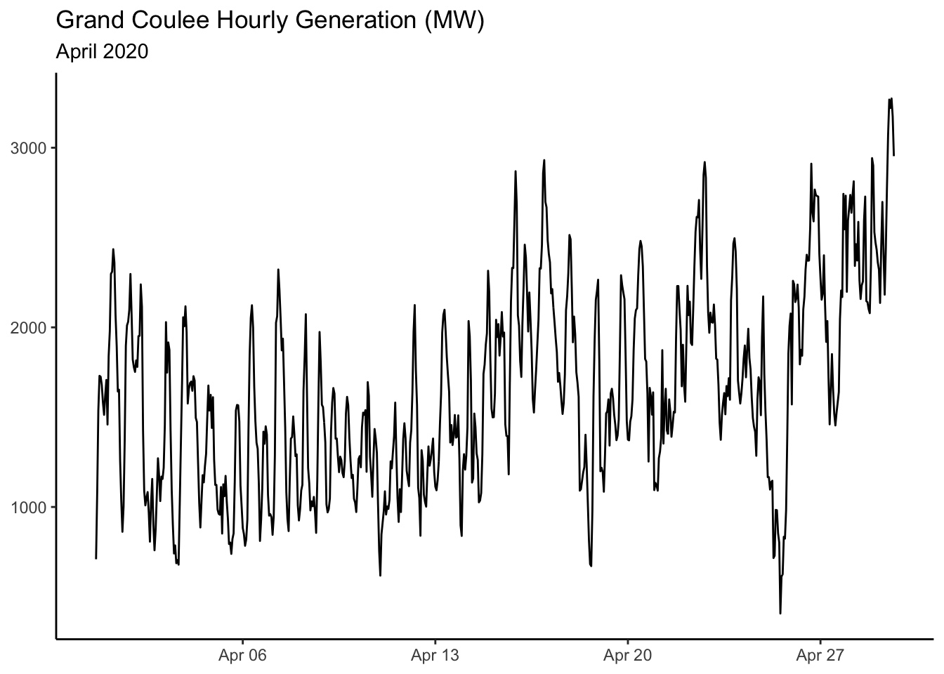

2. USBR powered flow records (Upper Colorado)

For the Upper Colorado I’m first gonna scrape a metadata file that tells me which dams actually have power releases available…

vroom("https://www.usbr.gov/uc/water/hydrodata/reservoir_data/meta.csv") %>% 
  filter(datatype_metadata.datatype_common_name == "power release") %>% 
  select(data_id = site_datatype_id,
         site = site_metadata.site_common_name) ->
  all_sites_with_power

all_sites_with_power

## # A tibble: 10 x 2
##    data_id site         
##      <dbl> <chr>        
##  1    1857 BLUE MESA    
##  2    1858 MORROW POINT 
##  3    1859 CRYSTAL      
##  4    1860 FONTENELLE   
##  5    1861 FLAMING GORGE
##  6    1862 LAKE POWELL  
##  7    1864 PINEVIEW     
##  8    1865 DEER CREEK   
##  9    2217 NAVAJO       
## 10   21264 JORDANELLE

So we have hourly data for ten dams. Let’s get all of ’em at the same time using purrr::pmap

data_url_start <- "https://www.usbr.gov/pn-bin/hdb/hdb.pl?svr=uchdb2&sdi="
data_url_end <- "&tstp=HR&t1=2020-04-01T00:00&t2=2020-04-30T00:00&table=R&mrid=0&format=88"

library(purrr)

all_sites_with_power %>% 
  pmap_dfr(
    function(data_id, site){
      vroom(paste0(
        data_url_start, data_id, data_url_end
      ), col_types = cols(), delim = ",") -> x
      names(x) <- c("date_time", "Average_Power_Release_CFS")
      x %>% mutate(date_time = mdy_hm(date_time),
                   dam = site)
    }
      ) -> powered_releases_all_dams

Now plot…

powered_releases_all_dams %>% 
  ggplot(aes(date_time, Average_Power_Release_CFS)) +
  geom_line() + facet_wrap(~dam, scales = "free", ncol = 2) +
  theme_classic() + labs(x = NULL)

## Warning: Removed 1394 row(s) containing missing values (geom_path).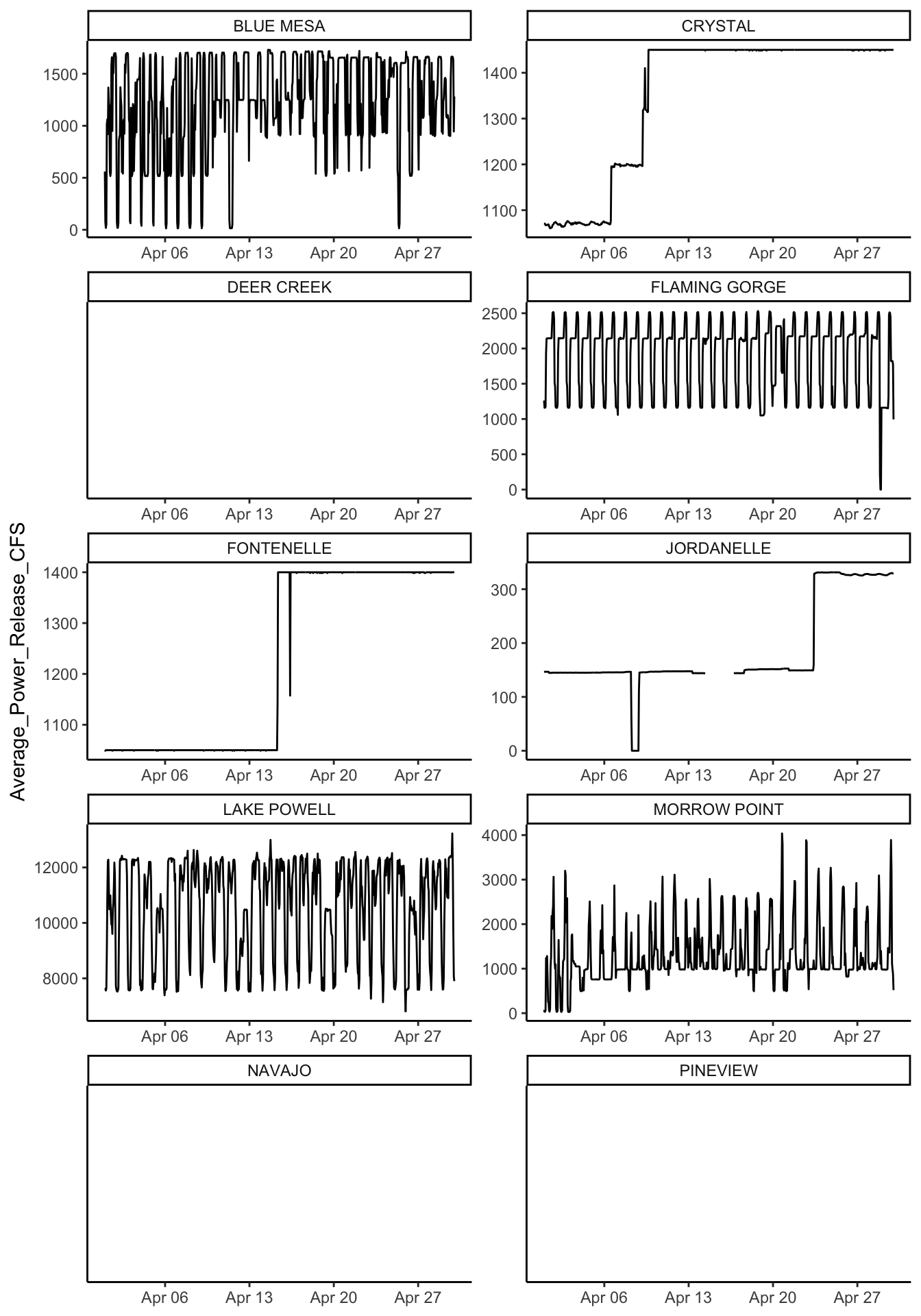

Ok, so it looks like a bunch are missing data for last month, but dig deeper into history and you’ll find data for all these sites going years back.

Enjoy.